Overview
The goal of DPMM is to fit a Dirichlet Process Mixture
Model to a dataset with continuous and/or categorical predictors. The
fitted model can be used for prediction of missing predictors.
In this file, we will analyse several datasets and show the capability of this package.
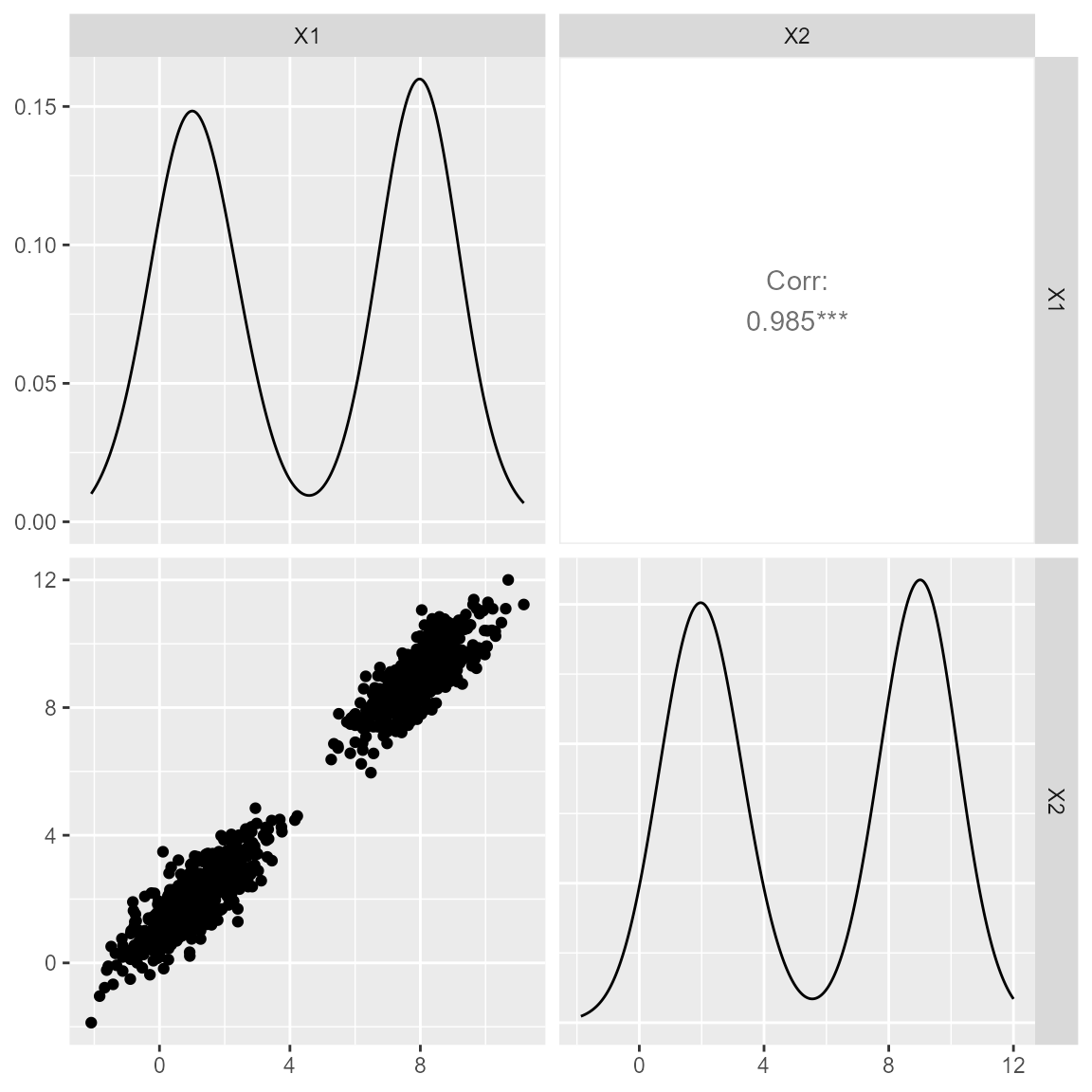
Dataset 1
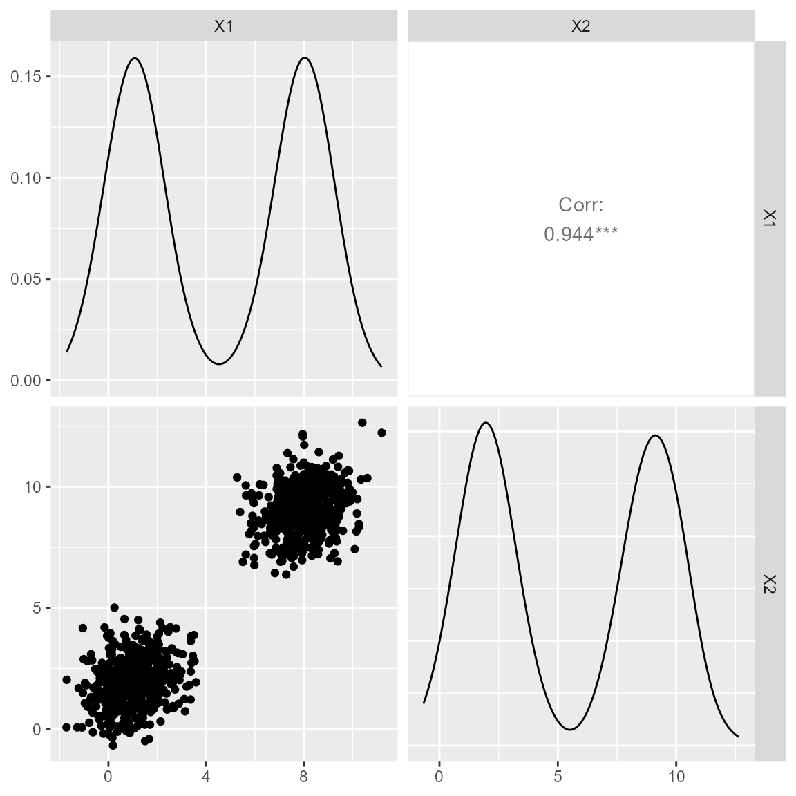
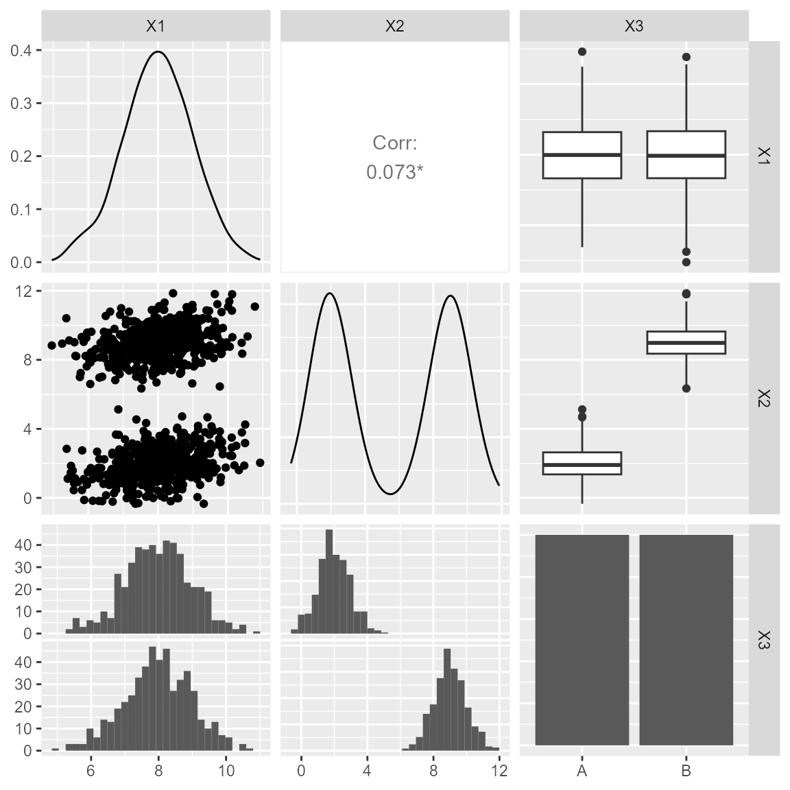
Dataset 1 is comprised of two distinct clusters, where the values of both predictor variables do not overlap each other. Therefore, one variable is informative of the other.
Example 1
We can fit the DPMM to the complete dataset. The ‘mcmc_iterations’ represents how long the MCMC chain should run (longer is better), ‘L’ represents the number of clusters that should be fitted, ‘mcmc_chain’ represents the number of MCMC chains being fitted in this function and ‘standardise’ chooses whether the continuous values should be standardised.
posteriors <- runModel(dataset_1,
                       mcmc_iterations = 2500,
                       L = 6,
                       mcmc_chains = 2,
                       standardise = TRUE)
#> ===== Monitors =====
#> thin = 1: alpha, logDens, muL, tauL, v, z
#> ===== Samplers =====
#> sumLogPostDens sampler (1)
#>   - logDens
#> RW_wishart sampler (1)
#>   - R1[1:2, 1:2]
#> RW sampler (2)
#>   - alpha
#>   - kappa1
#> conjugate sampler (17)
#>   - v[]  (5 elements)
#>   - muL[]  (6 multivariate elements)
#>   - tauL[]  (6 multivariate elements)
#> categorical sampler (1000)
#>   - z[]  (1000 elements)
#> |-------------|-------------|-------------|-------------|
#> |-------------------------------------------------------|
#> |-------------|-------------|-------------|-------------|
#> |-------------------------------------------------------|
We can check the fit of the DPMM to ensure that random samples from the fitted DPMM are in the same covariate space as the original data.
plot_ggpairs(posteriors,
             newdata = dataset_1,
             nburn = 1500)
We can introduce missingness in the dataset and check whether the DPMM is predicting values in the right cluster. In this case, we introduce missingness in ‘X1’ for some of the patients in one of the clusters.
rows <- 1:50
dataset_missing <- dataset_1
dataset_missing_predict <- dataset_missing[rows,]
dataset_missing_predict[,"X1"] <- as.numeric(NA)
And make predictions from the fitted DPMM.
posteriors.prediction <- predict_dpmm_fit(posteriors,
                                          newdata = dataset_missing_predict,
                                          samples = seq(1500,2500, 25))
We can then check whether the values are being predicted in the right place. First, we calculate the credible intervals for each predicted value.
low_q <- NULL
median_q <- NULL
high_q <- NULL
for (i in 1:length(posteriors.prediction)) {
  low_q <- c(low_q, quantile(unlist(posteriors.prediction[[i]][]), probs = c(0.05)))
  median_q <- c(median_q, quantile(unlist(posteriors.prediction[[i]][]), probs = c(0.5)))
  high_q <- c(high_q, quantile(unlist(posteriors.prediction[[i]][]), probs = c(0.95)))
}
We then standardise the original values to match the standardisation in the DPMM.
standardised_values <- (dataset_missing[rows,"X1"]-posteriors$mean_values[1])/posteriors$sd_values[1]Lastly, we plot the credible intervals against the true values.
cbind(standardised_values,low_q, median_q,high_q) %>%
  as.data.frame() %>%
   rlang::set_names(c("observed", "low","median","high")) %>%
  ggplot() +
  geom_point(aes(x = observed, y = median)) +
  geom_errorbar(aes(x = observed, ymin = low, ymax = high)) +
  geom_abline(aes(intercept = 0, slope = 1))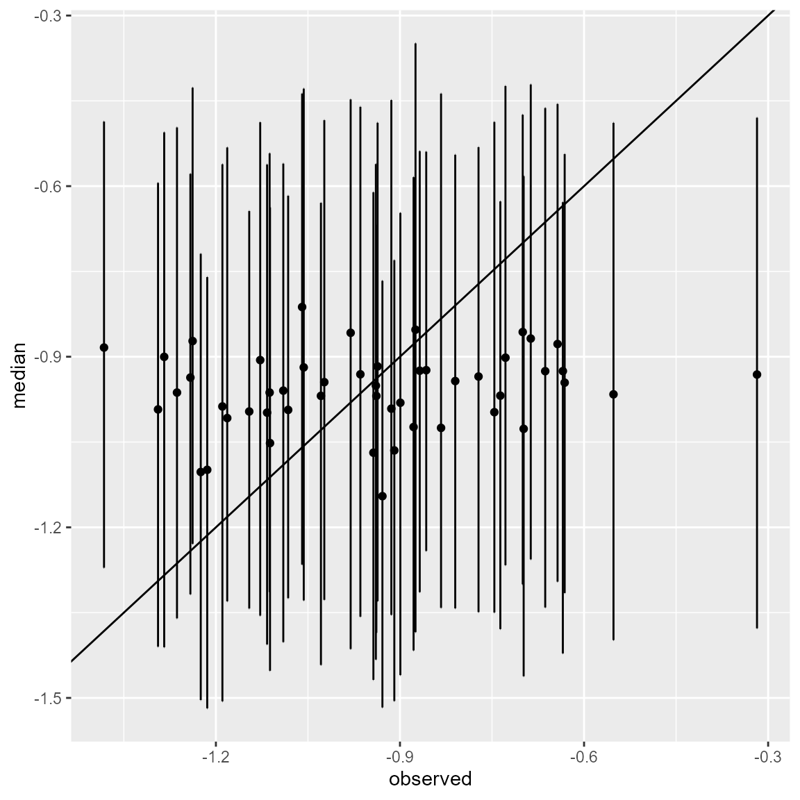
Example 2
We can also fit the model without standardising.
posteriors <- runModel(dataset_1,
                       mcmc_iterations = 2500,
                       L = 6,
                       mcmc_chains = 2,
                       standardise = FALSE)
#> ===== Monitors =====
#> thin = 1: alpha, logDens, muL, tauL, v, z
#> ===== Samplers =====
#> sumLogPostDens sampler (1)
#>   - logDens
#> RW_wishart sampler (1)
#>   - R1[1:2, 1:2]
#> RW sampler (2)
#>   - alpha
#>   - kappa1
#> conjugate sampler (17)
#>   - v[]  (5 elements)
#>   - muL[]  (6 multivariate elements)
#>   - tauL[]  (6 multivariate elements)
#> categorical sampler (1000)
#>   - z[]  (1000 elements)
#> |-------------|-------------|-------------|-------------|
#> |-------------------------------------------------------|
#> |-------------|-------------|-------------|-------------|
#> |-------------------------------------------------------|
We can check the fit of the DPMM.
plot_ggpairs(posteriors, dataset_1, nburn = 1500)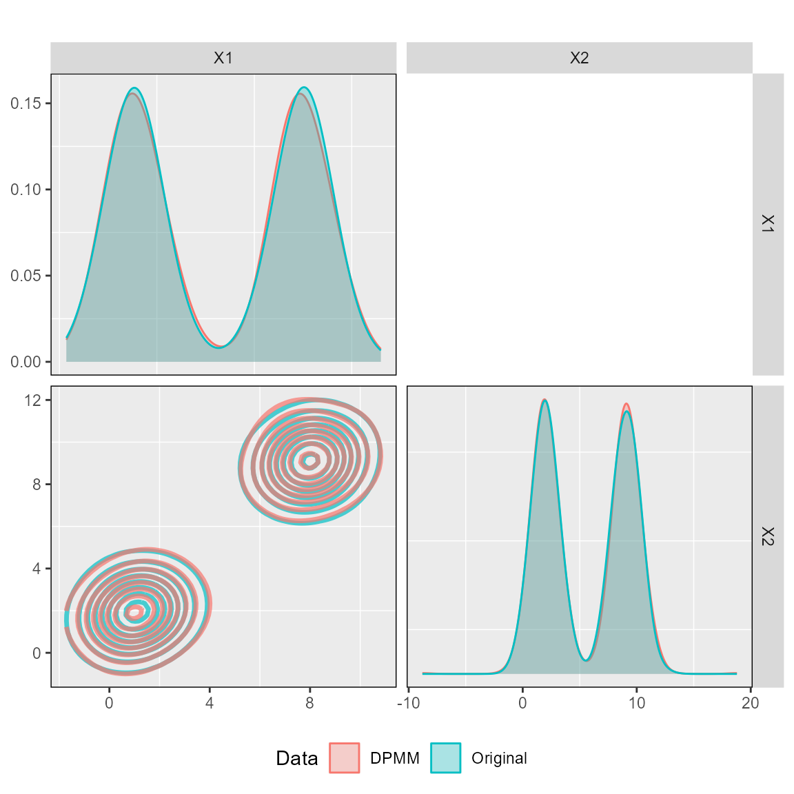
We then use the same dataset to make prediction from the newly fitted DPMM.
posteriors.prediction <- predict_dpmm_fit(posteriors,
                                          newdata = dataset_missing_predict,
                                          samples = seq(1500,2500, 25))
And, once again, check whether the credible intervals are close to the original values.
low_q <- NULL
median_q <- NULL
high_q <- NULL
for (i in 1:length(posteriors.prediction)) {
  low_q <- c(low_q, quantile(unlist(posteriors.prediction[[i]][]), probs = c(0.05)))
  median_q <- c(median_q, quantile(unlist(posteriors.prediction[[i]][]), probs = c(0.5)))
  high_q <- c(high_q, quantile(unlist(posteriors.prediction[[i]][]), probs = c(0.95)))
}

cbind(dataset_missing[1:50,"X1"],low_q, median_q,high_q) %>%
  as.data.frame() %>%
   rlang::set_names(c("observed", "low","median","high")) %>%
  ggplot() +
  geom_point(aes(x = observed, y = median)) +
  geom_errorbar(aes(x = observed, ymin = low, ymax = high)) +
  geom_abline(aes(intercept = 0, slope = 1))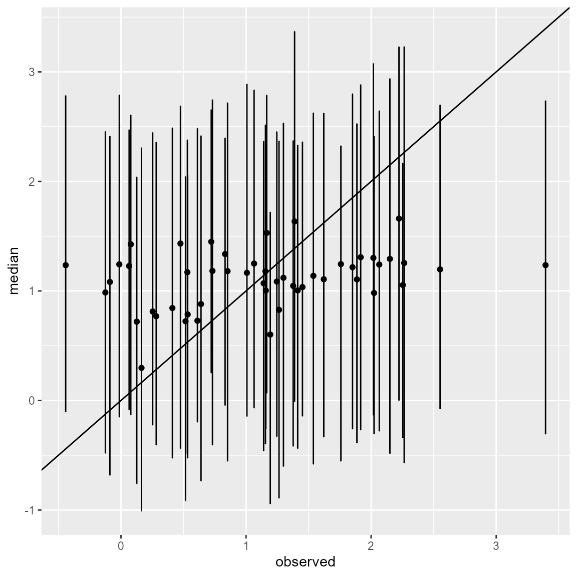
Example 3
We can also fit the DPMM with missing data present in the original dataset. Let’s introduce some misisngness in both clusters.
dataset_missing <- dataset_1
dataset_missing[1,"X1"] <- NA
dataset_missing[501,"X1"] <- NA
Then we fit the DPMM whilst standardising values.
posteriors <- runModel(dataset_missing,
mcmc_iterations = 2500,
L = 6,
mcmc_chains = 2,
standardise = TRUE)
#> ===== Monitors =====
#> thin = 1: alpha, logDens, muL, tauL, v, x_cont_miss, z
#> ===== Samplers =====
#> sumLogPostDens sampler (1)
#> - logDens
#> RW_wishart sampler (1)
#> - R1[1:2, 1:2]
#> RW sampler (2)
#> - alpha
#> - kappa1
#> conjugate sampler (17)
#> - v[] (5 elements)
#> - muL[] (6 multivariate elements)
#> - tauL[] (6 multivariate elements)
#> conditional_RW sampler (2)
#> - x_cont_miss[1, 1:2]
#> - x_cont_miss[2, 1:2]
#> categorical sampler (1000)
#> - z[] (998 elements)
#> - zmiss[] (2 elements)
#> |-------------|-------------|-------------|-------------|
#> |-------------------------------------------------------|
#> |-------------|-------------|-------------|-------------|
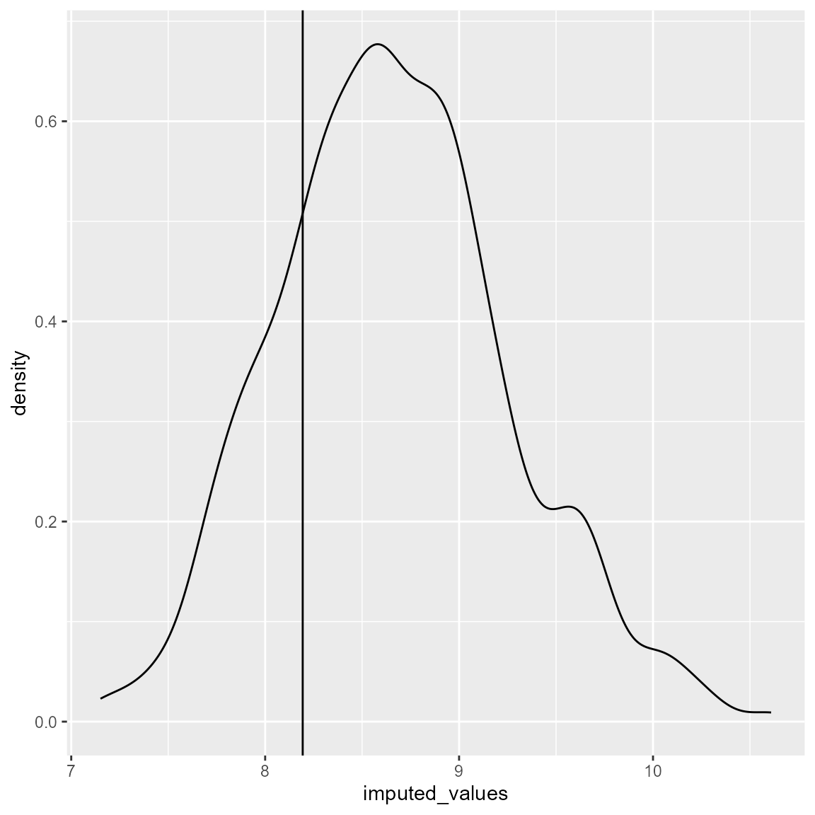
#> |-------------------------------------------------------|And we can check how well are those missing values being imputed during the model fitting. Here, we are only checking chain 1, but it can be repeated for all other chains.
intercept_1 = (dataset_1[1,"X1"]-posteriors$mean_values[1])/posteriors$sd_values[1]
ggplot() +
  geom_density(aes(x = as_tibble(posteriors$samples$chain1)%>%
                     select(`x_cont_miss[1, 1]`)%>%
                     dplyr::slice(1000:2500)%>%
                     unlist())) +
  geom_vline(aes(xintercept = intercept_1))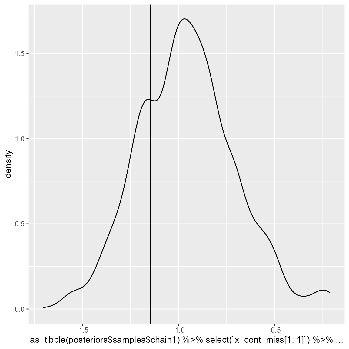
intercept_2 = (dataset_1[501,"X1"]-posteriors$mean_values[1])/posteriors$sd_values[1]
ggplot() +
  geom_density(aes(x = as_tibble(posteriors$samples$chain1)%>%
                     select(`x_cont_miss[2, 1]`)%>%
                     dplyr::slice(1000:2500)%>%
                     unlist())) +
  geom_vline(aes(xintercept = intercept_2))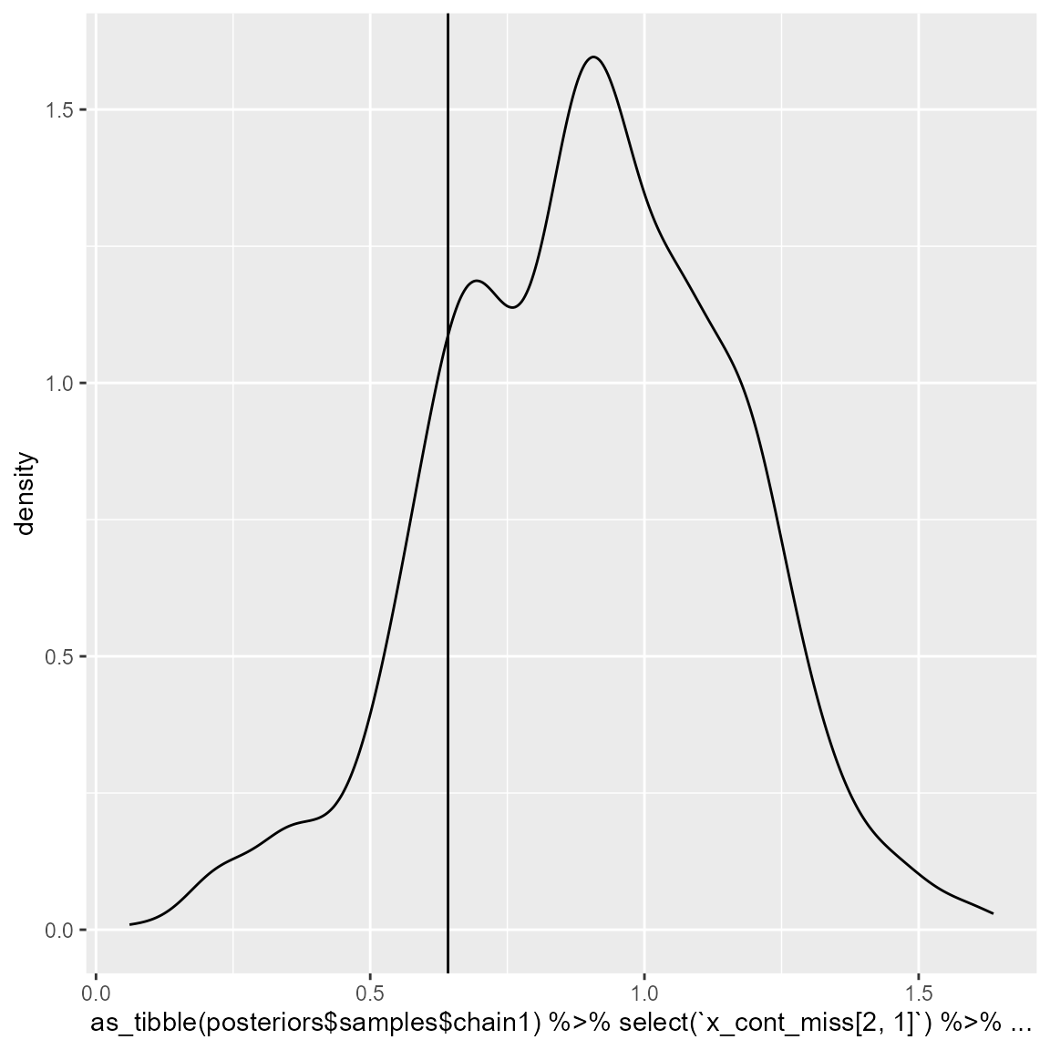
Example 4
The same exercise can be done again, but without standardising continuous values.
posteriors <- runModel(dataset_missing,
                       mcmc_iterations = 2500,
                       L = 6,
                       mcmc_chains = 2,
                       standardise = FALSE)
#> ===== Monitors =====
#> thin = 1: alpha, logDens, muL, tauL, v, x_cont_miss, z
#> ===== Samplers =====
#> sumLogPostDens sampler (1)
#>   - logDens
#> RW_wishart sampler (1)
#>   - R1[1:2, 1:2]
#> RW sampler (2)
#>   - alpha
#>   - kappa1
#> conjugate sampler (17)
#>   - v[]  (5 elements)
#>   - muL[]  (6 multivariate elements)
#>   - tauL[]  (6 multivariate elements)
#> conditional_RW sampler (2)
#>   - x_cont_miss[1, 1:2]
#>   - x_cont_miss[2, 1:2]
#> categorical sampler (1000)
#>   - z[]  (998 elements)
#>   - zmiss[]  (2 elements)
#> |-------------|-------------|-------------|-------------|
#> |-------------------------------------------------------|
#> |-------------|-------------|-------------|-------------|
#> |-------------------------------------------------------|
And we check the values imputed.
ggplot() +
  geom_density(aes(x = as_tibble(posteriors$samples$chain1)%>%
                     select(`x_cont_miss[1, 1]`)%>%
                     dplyr::slice(1000:2500)%>%
                     unlist())) +
  geom_vline(aes(xintercept = dataset_1[1,"X1"]))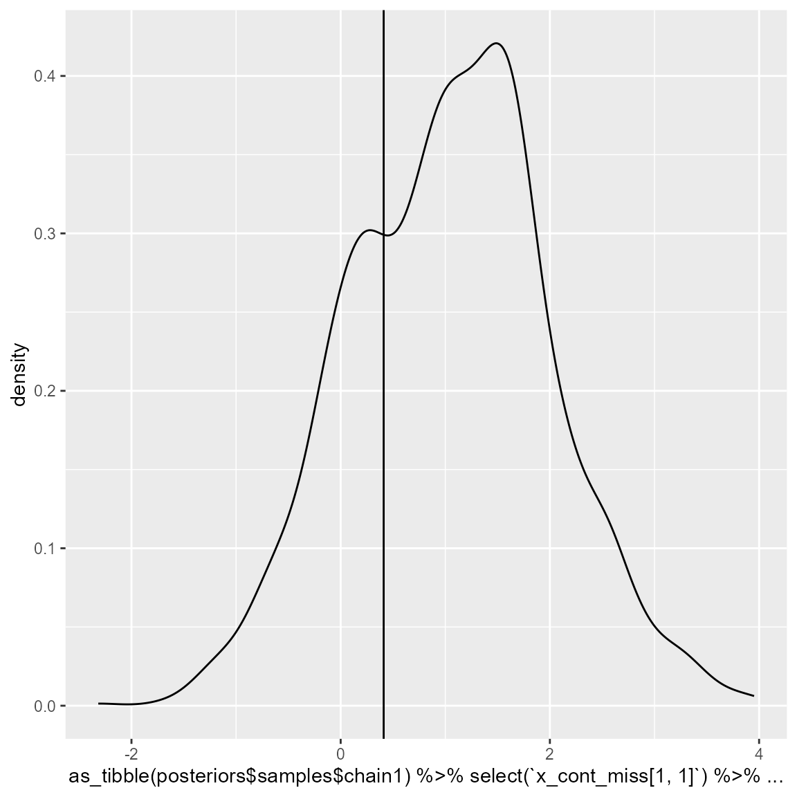
ggplot() +
  geom_density(aes(x = as_tibble(posteriors$samples$chain1)%>%
                     select(`x_cont_miss[2, 1]`)%>%
                     dplyr::slice(1000:2500)%>%
                     unlist())) +
  geom_vline(aes(xintercept = dataset_1[501,"X1"]))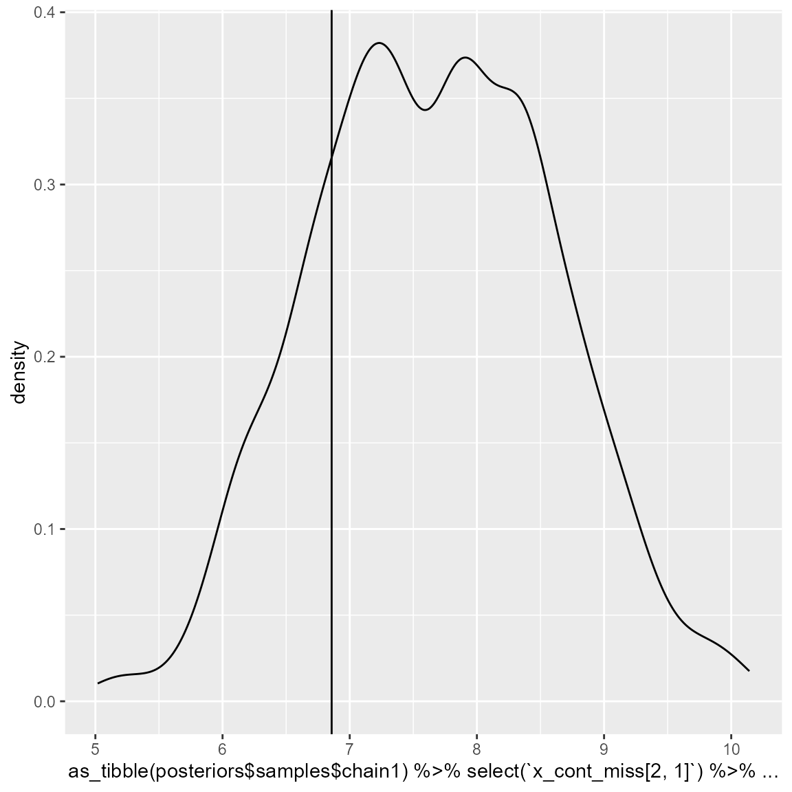
Dataset 2
Dataset 2 is comprised of two distinct clusters, where the values of ‘X2’ and ‘X3’ are informative of the cluster membership, but not ‘X1’.
Example 1
We can fit the DPMM to the complete dataset.
posteriors <- runModel(dataset_2,
mcmc_iterations = 2500,
L = 6,
mcmc_chains = 2)
#> ===== Monitors =====
#> thin = 1: alpha, logDens, muL, phiL, tauL, v, z
#> ===== Samplers =====
#> sumLogPostDens sampler (1)
#> - logDens
#> RW_wishart sampler (1)
#> - R1[1:2, 1:2]
#> RW sampler (2)
#> - alpha
#> - kappa1
#> conjugate sampler (23)
#> - v[] (5 elements)
#> - phiL[] (6 multivariate elements)
#> - muL[] (6 multivariate elements)
#> - tauL[] (6 multivariate elements)
#> categorical sampler (1000)
#> - z[] (1000 elements)
#> |-------------|-------------|-------------|-------------|
#> |-------------------------------------------------------|
#> |-------------|-------------|-------------|-------------|
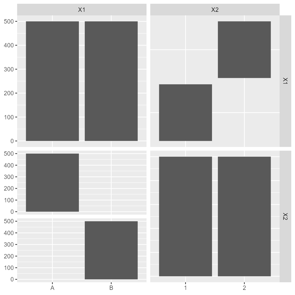
#> |-------------------------------------------------------|We then check the fit of the DPMM versus the original data.
plot_ggpairs(posteriors,
             newdata = dataset_2,
             nburn = 1500)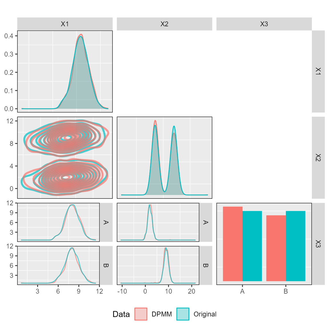
We can introduce missingness in the dataset and check whether the DPMM is predicting values in the right cluster. In this case, we introduce missingness in ‘X2’ for some of the patients in one of the clusters.
rows <- 950:1000
dataset_missing <- dataset_2
dataset_missing_predict <- dataset_missing[rows,]
dataset_missing_predict[,"X2"] <- as.numeric(NA)
And make predictions from the fitted DPMM.
posteriors.prediction <- predict_dpmm_fit(posteriors,
                                          newdata = dataset_missing_predict,
                                          samples = seq(1500,2500, 25))
We can then check whether the values are being predicted in the right place.
low_q <- NULL
median_q <- NULL
high_q <- NULL
for (i in 1:length(posteriors.prediction)) {
  low_q <- c(low_q, quantile(unlist(posteriors.prediction[[i]][]), probs = c(0.05)))
  median_q <- c(median_q, quantile(unlist(posteriors.prediction[[i]][]), probs = c(0.5)))
  high_q <- c(high_q, quantile(unlist(posteriors.prediction[[i]][]), probs = c(0.95)))
}
We then standardise the original values to match the standardisation in the DPMM.
standardised_values <- (dataset_missing[rows,"X2"]-posteriors$mean_values[2])/posteriors$sd_values[2]Lastly, we plot the credible intervals against the true values.
cbind(standardised_values,low_q, median_q,high_q) %>%
  as.data.frame() %>%
   rlang::set_names(c("observed", "low","median","high")) %>%
  ggplot() +
  geom_point(aes(x = observed, y = median)) +
  geom_errorbar(aes(x = observed, ymin = low, ymax = high)) +
  geom_abline(aes(intercept = 0, slope = 1))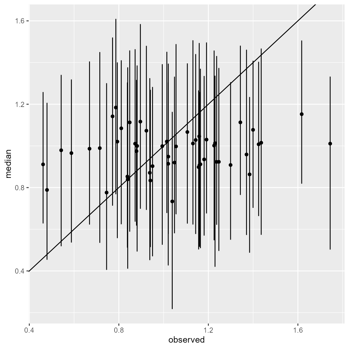
Example 2
We can do the same exercise but adding missingness to ‘X3’ instead.
rows <- 950:1000
dataset_missing <- dataset_2
dataset_missing_predict <- dataset_missing[rows,]
dataset_missing_predict[,"X3"] <- factor(NA, levels = levels(dataset_2[,"X3"]))
And make predictions from the fitted DPMM.
posteriors.prediction <- predict_dpmm_fit(posteriors,
                                          newdata = dataset_missing_predict,
                                          samples = seq(1500,2500, 25))
We can then check whether the values are being predicted in the right place by plotting a table of the original values versus the predicted values.
predicted <- NULL
for (i in 1:length(posteriors.prediction)) {
  var <- table(unlist(posteriors.prediction[i]))
  predicted <- c(predicted, names(var[var==max(var)]))
}
predicted <- as.numeric(predicted)

cbind(dataset_2[rows,"X3"],predicted) %>%
  as.data.frame() %>%
   rlang::set_names(c("observed", "predicted")) %>%
  mutate(observed = factor(observed),
         predicted = factor(predicted)) %>%
  table()
#>         predicted
#> observed  2
#>        2 51
Example 3
We can also fit the DPMM with missing data in ‘X3’ present in the original dataset. Let’s introduce some misisngness in both clusters.
dataset_missing <- dataset_2
dataset_missing[2,"X3"] <- NA
dataset_missing[501,"X3"] <- NA
Then we fit the DPMM whilst standardising values.
posteriors <- runModel(dataset_missing,
                       mcmc_iterations = 2500,
                       L = 6,
                       standardise = FALSE)
#> ===== Monitors =====
#> thin = 1: alpha, logDens, muL, phiL, tauL, v, x_disc_miss, z
#> ===== Samplers =====
#> sumLogPostDens sampler (1)
#>   - logDens
#> RW_wishart sampler (1)
#>   - R1[1:2, 1:2]
#> RW sampler (2)
#>   - alpha
#>   - kappa1
#> posterior_predictive sampler (2)
#>   - x_disc_miss[]  (2 elements)
#> conjugate sampler (23)
#>   - v[]  (5 elements)
#>   - phiL[]  (6 multivariate elements)
#>   - muL[]  (6 multivariate elements)
#>   - tauL[]  (6 multivariate elements)
#> categorical sampler (1000)
#>   - z[]  (998 elements)
#>   - zmiss[]  (2 elements)
#> |-------------|-------------|-------------|-------------|
#> |-------------------------------------------------------|
#> |-------------|-------------|-------------|-------------|
#> |-------------------------------------------------------|
And we can check how well are those missing values being imputed during the model fitting. Here, we are only checking chain 1, but it can be repeated for all other chains.
imputed_values <- as_tibble(posteriors$samples$chain1)%>%
  select(`x_disc_miss[1, 1]`)%>%
  dplyr::slice(1000:2500)%>%
  unlist()
cbind(imputed_values, rep(as.numeric(dataset_2[2,"X3"]), 1501)) %>%
  as.data.frame() %>%
   rlang::set_names(c("Predicted","True")) %>%
  table()
#>          True
#> Predicted    1
#>         1 1499
#>         2    2

imputed_values <- as_tibble(posteriors$samples$chain1)%>%
  select(`x_disc_miss[2, 1]`)%>%
  dplyr::slice(1000:2500)%>%
  unlist()
cbind(imputed_values, rep(as.numeric(dataset_2[501,"X3"]), 1501)) %>%
  as.data.frame() %>%
   rlang::set_names(c("Predicted","True")) %>%
  table()
#>          True
#> Predicted    2
#>         1    1
#>         2 1500
Example 4
We can also fit the DPMM with missing data in “X2” present in the original dataset. Let’s introduce some misisngness in both clusters.
dataset_missing <- dataset_2
dataset_missing[1,"X2"] <- NA
dataset_missing[501,"X2"] <- NA
Then we fit the DPMM whilst standardising values.
posteriors <- runModel(dataset_missing,
                       mcmc_iterations = 2500,
                       L = 6,
                       standardise = FALSE)
#> ===== Monitors =====
#> thin = 1: alpha, logDens, muL, phiL, tauL, v, x_cont_miss, z
#> ===== Samplers =====
#> sumLogPostDens sampler (1)
#>   - logDens
#> RW_wishart sampler (1)
#>   - R1[1:2, 1:2]
#> RW sampler (2)
#>   - alpha
#>   - kappa1
#> conjugate sampler (23)
#>   - v[]  (5 elements)
#>   - phiL[]  (6 multivariate elements)
#>   - muL[]  (6 multivariate elements)
#>   - tauL[]  (6 multivariate elements)
#> conditional_RW sampler (2)
#>   - x_cont_miss[1, 1:2]
#>   - x_cont_miss[2, 1:2]
#> categorical sampler (1000)
#>   - z[]  (998 elements)
#>   - zmiss[]  (2 elements)
#> |-------------|-------------|-------------|-------------|
#> |-------------------------------------------------------|
#> |-------------|-------------|-------------|-------------|
#> |-------------------------------------------------------|
And we can check how well are those missing values being imputed during the model fitting. Here, we are only checking chain 1, but it can be repeated for all other chains.
imputed_values <- as_tibble(posteriors$samples$chain1)%>%
  select(`x_cont_miss[1, 2]`)%>%
  dplyr::slice(1000:2500)%>%
  unlist()
ggplot() +
  geom_density(aes(x = imputed_values)) +
  geom_vline(aes(xintercept = dataset_2[1,"X2"]))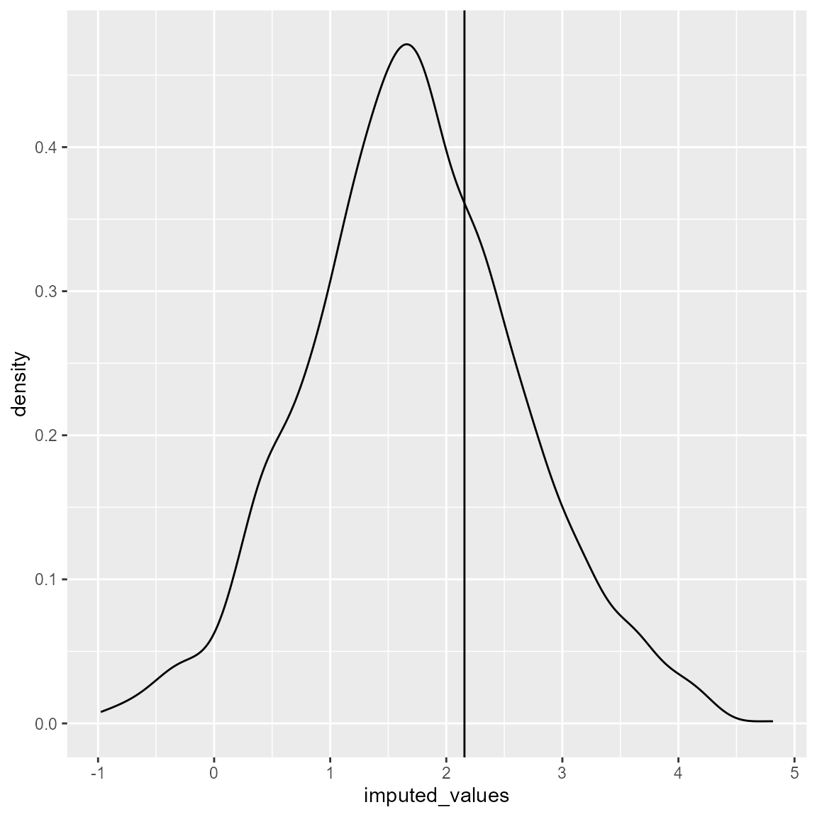
imputed_values <- as_tibble(posteriors$samples$chain1)%>%
  select(`x_cont_miss[2, 2]`)%>%
  dplyr::slice(1000:2500)%>%
  unlist()
ggplot() +
  geom_density(aes(x = imputed_values)) +
  geom_vline(aes(xintercept = dataset_2[501,"X2"]))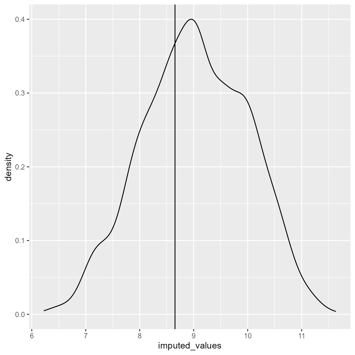
Example 5
We can also fit the DPMM with missing data in “X1” and “X2” present in the original dataset. Let’s introduce some misisngness in both clusters.
Then we fit the DPMM whilst standardising values.
posteriors <- runModel(dataset_missing,
                       mcmc_iterations = 2500,
                       L = 6,
                       standardise = FALSE)
#> ===== Monitors =====
#> thin = 1: alpha, logDens, muL, phiL, tauL, v, x_cont_miss, z
#> ===== Samplers =====
#> sumLogPostDens sampler (1)
#>   - logDens
#> RW_wishart sampler (1)
#>   - R1[1:2, 1:2]
#> RW sampler (2)
#>   - alpha
#>   - kappa1
#> posterior_predictive sampler (2)
#>   - x_cont_miss[1, 1:2]
#>   - x_cont_miss[2, 1:2]
#> conjugate sampler (23)
#>   - v[]  (5 elements)
#>   - phiL[]  (6 multivariate elements)
#>   - muL[]  (6 multivariate elements)
#>   - tauL[]  (6 multivariate elements)
#> categorical sampler (1000)
#>   - z[]  (998 elements)
#>   - zmiss[]  (2 elements)
#> |-------------|-------------|-------------|-------------|
#> |-------------------------------------------------------|
#> |-------------|-------------|-------------|-------------|
#> |-------------------------------------------------------|
And we can check how well are those missing values being imputed during the model fitting. Here, we are only checking chain 1, but it can be repeated for all other chains.
ggplot() +
  geom_point(aes(x = as_tibble(posteriors$samples$chain1)%>%
                   select(`x_cont_miss[1, 1]`)%>%
                   dplyr::slice(1000:2500)%>%
                   unlist(),
                 y = as_tibble(posteriors$samples$chain1)%>%
                   select(`x_cont_miss[1, 2]`)%>%
                   dplyr::slice(1000:2500)%>%
                   unlist()), colour = "darkorange") +
  geom_point(aes(x = dataset_2[1,"X1"], y = dataset_2[1,"X2"]),
             colour = "darkorange3",
             fill = "black",
             size = 3) +
  geom_point(aes(x = as_tibble(posteriors$samples$chain1)%>%
                   select(`x_cont_miss[2, 1]`)%>%
                   dplyr::slice(1000:2500)%>%
                   unlist(),
                 y = as_tibble(posteriors$samples$chain1)%>%
                   select(`x_cont_miss[2, 2]`)%>%
                   dplyr::slice(1000:2500)%>%
                   unlist()), colour = "royalblue") +
  geom_point(aes(x = dataset_2[501,"X1"], y = dataset_2[501,"X2"]),
             colour = "royalblue4",
             fill = "black",
             size = 3)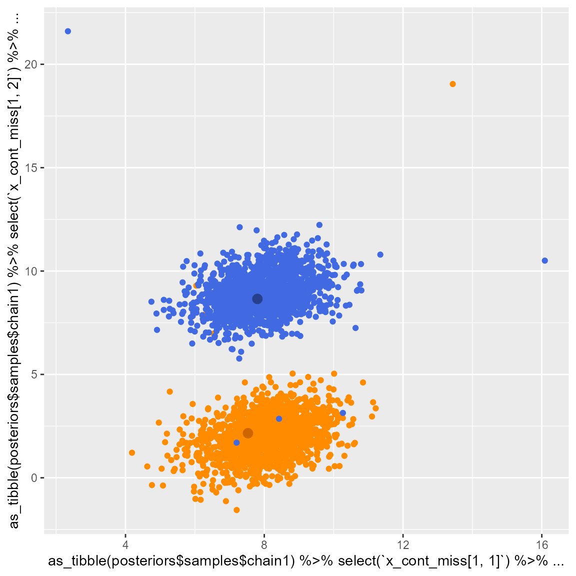
Dataset 3
Dataset 3 is comprised of two distinct clusters, where the values of ‘X1’ and ‘X2’ are informative of the cluster membership.
Example 1
We can fit the DPMM to the complete dataset.
posteriors <- runModel(dataset_3,
                       mcmc_iterations = 2500,
                       L = 6,
                       mcmc_chains = 2)
#> ===== Monitors =====
#> thin = 1: alpha, logDens, phiL, v, z
#> ===== Samplers =====
#> sumLogPostDens sampler (1)
#>   - logDens
#> RW sampler (1)
#>   - alpha
#> conjugate sampler (17)
#>   - v[]  (5 elements)
#>   - phiL[]  (12 multivariate elements)
#> categorical sampler (1000)
#>   - z[]  (1000 elements)
#> |-------------|-------------|-------------|-------------|
#> |-------------------------------------------------------|
#> |-------------|-------------|-------------|-------------|
#> |-------------------------------------------------------|
We then check the fit of the DPMM versus the original data.
## PROBLEM HERE
plot_ggpairs(posteriors,
             newdata = dataset_3,
             nburn = 1500)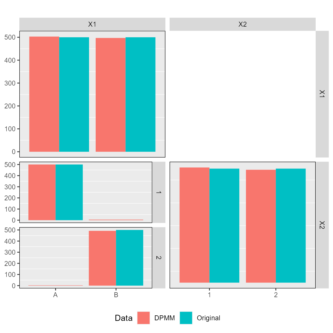
We can introduce missingness in the dataset and check whether the DPMM is predicting values in the right cluster. In this case, we introduce missingness in ‘X2’ for some of the patients in one of the clusters.
rows <- 950:1000
dataset_missing <- dataset_3
dataset_missing_predict <- dataset_missing[rows,]
dataset_missing_predict[,"X1"] <- factor(NA, levels = levels(dataset_3[,"X1"]))
And make predictions from the fitted DPMM.
posteriors.prediction <- predict_dpmm_fit(posteriors,
                                          newdata = dataset_missing_predict,
                                          samples = seq(1500,2500, 25))
We can then check whether the values are being predicted in the right place.
predicted <- NULL
for (i in 1:length(posteriors.prediction)) {
  var <- table(unlist(posteriors.prediction[i]))
  predicted <- c(predicted, names(var[var==max(var)]))
}
predicted <- as.numeric(predicted)

cbind(dataset_3[rows,"X1"],predicted) %>%
  as.data.frame() %>%
   rlang::set_names(c("observed", "predicted")) %>%
  mutate(observed = factor(observed),
         predicted = factor(predicted)) %>%
  table()
#>         predicted
#> observed  2
#>        2 51
Example 2
We can also fit the DPMM with missing data in “X1” present in the original dataset. Let’s introduce some misisngness in both clusters.
dataset_missing <- dataset_3
dataset_missing[1,"X1"] <- factor(NA, levels = levels(dataset_3[,"X1"]))
dataset_missing[501,"X1"] <- factor(NA, levels = levels(dataset_3[,"X1"]))
Then we fit the DPMM whilst standardising values.
posteriors <- runModel(dataset_missing,
                       mcmc_iterations = 2500,
                       L = 6,
                       standardise = FALSE)
#> ===== Monitors =====
#> thin = 1: alpha, logDens, phiL, v, x_disc_miss, z
#> ===== Samplers =====
#> sumLogPostDens sampler (1)
#>   - logDens
#> RW sampler (1)
#>   - alpha
#> posterior_predictive sampler (2)
#>   - x_disc_miss[]  (2 elements)
#> conjugate sampler (17)
#>   - v[]  (5 elements)
#>   - phiL[]  (12 multivariate elements)
#> categorical sampler (1000)
#>   - z[]  (998 elements)
#>   - zmiss[]  (2 elements)
#> |-------------|-------------|-------------|-------------|
#> |-------------------------------------------------------|
#> |-------------|-------------|-------------|-------------|
#> |-------------------------------------------------------|
And we can check how well are those missing values being imputed during the model fitting. Here, we are only checking chain 1, but it can be repeated for all other chains.
imputed_values <- as_tibble(posteriors$samples$chain1)%>%
  select(`x_disc_miss[1, 1]`)%>%
  dplyr::slice(1000:2500)%>%
  unlist()
cbind(imputed_values, dataset_3[1,"X1"]) %>%
  as.data.frame() %>%
   rlang::set_names(c("Prediction","True Value")) %>%
  table()
#>           True Value
#> Prediction    1
#>          1 1495
#>          2    6

imputed_values <- as_tibble(posteriors$samples$chain1)%>%
  select(`x_disc_miss[2, 1]`)%>%
  dplyr::slice(1000:2500)%>%
  unlist()
cbind(imputed_values, dataset_3[501,"X1"]) %>%
  as.data.frame() %>%
   rlang::set_names(c("Prediction","True Value")) %>%
  table()
#>           True Value
#> Prediction    2
#>          1    9
#>          2 1492
Dataset 4
Dataset 4 is comprised of a ‘Y’ outcome variable, ‘X1’/‘X2’/‘X3’ continuous predictors and ‘X4’ categorical predictor.
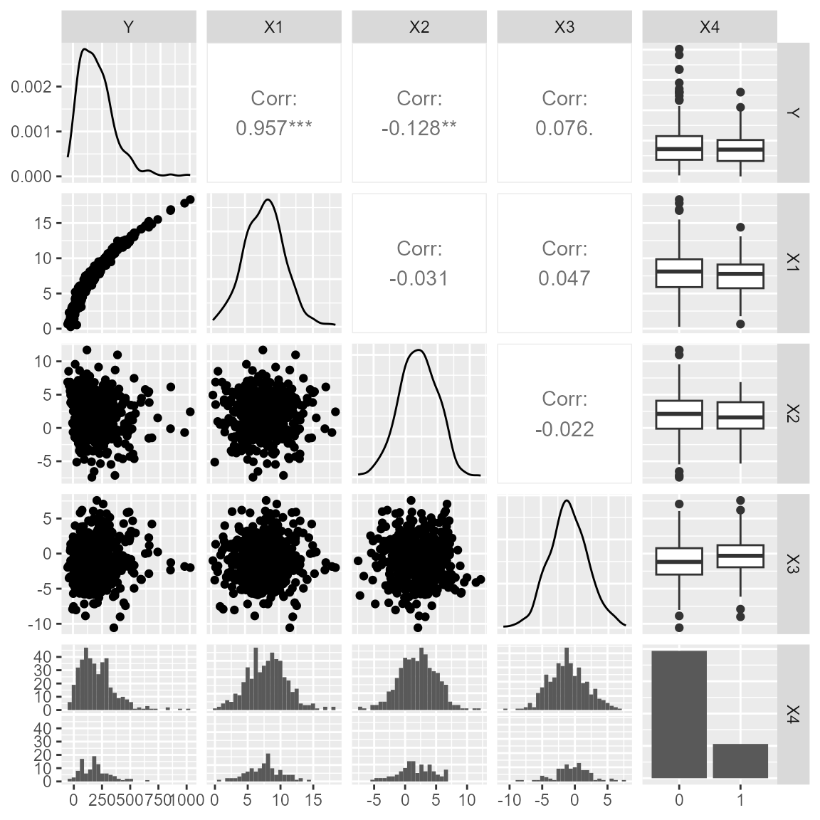
Example 1
We can fit the DPMM to the complete dataset.
posteriors <- runModel(dataset_4,
                       mcmc_iterations = 2500,
                       L = 6,
                       standardise = FALSE)
#> ===== Monitors =====
#> thin = 1: alpha, logDens, muL, phiL, tauL, v, z
#> ===== Samplers =====
#> sumLogPostDens sampler (1)
#>   - logDens
#> RW_wishart sampler (1)
#>   - R1[1:4, 1:4]
#> RW sampler (2)
#>   - alpha
#>   - kappa1
#> conjugate sampler (23)
#>   - v[]  (5 elements)
#>   - phiL[]  (6 multivariate elements)
#>   - muL[]  (6 multivariate elements)
#>   - tauL[]  (6 multivariate elements)
#> categorical sampler (500)
#>   - z[]  (500 elements)
#> |-------------|-------------|-------------|-------------|
#> |-------------------------------------------------------|
#> |-------------|-------------|-------------|-------------|
#> |-------------------------------------------------------|
We then check the fit of the DPMM versus the original data.
plot_ggpairs(posteriors,
             newdata = dataset_4,
             nburn = 1500)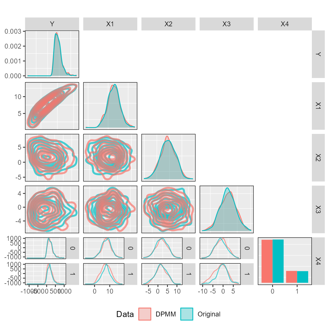
We can introduce missingness in the dataset and check whether the DPMM is predicting values correctly. In this case, we introduce missingness in ‘Y’ for 100 random patients.
rows <- sample(1:nrow(dataset_4), 100)
dataset_missing <- dataset_4
dataset_missing_predict <- dataset_missing[rows,]
dataset_missing_predict[,"Y"] <- as.numeric(NA)
And make predictions from the fitted DPMM.
posteriors.prediction <- predict_dpmm_fit(posteriors,
                                          dataset_missing_predict,
                                          samples = seq(1500,2500, 25))
We can then check whether the values are being predicted in the right place.
low_q <- NULL
median_q <- NULL
high_q <- NULL
for (i in 1:length(posteriors.prediction)) {
  low_q <- c(low_q, quantile(unlist(posteriors.prediction[[i]][]), probs = c(0.05)))
  median_q <- c(median_q, quantile(unlist(posteriors.prediction[[i]][]), probs = c(0.5)))
  high_q <- c(high_q, quantile(unlist(posteriors.prediction[[i]][]), probs = c(0.95)))
}

cbind(dataset_4[rows,"Y"],low_q, median_q,high_q) %>%
  as.data.frame() %>%
   rlang::set_names(c("observed", "low","median","high")) %>%
  ggplot() +
  geom_point(aes(x = observed, y = median)) +
  geom_errorbar(aes(x = observed, ymin = low, ymax = high)) +
  geom_abline(aes(intercept = 0, slope = 1))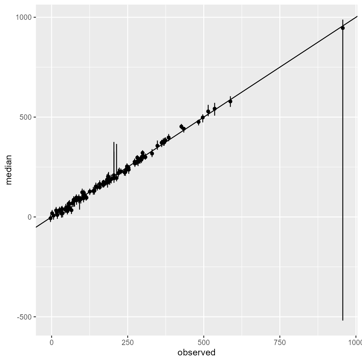
Dataset 5
Dataset 5 is comprised of two distinct clusters, where the values of ‘X1’ overlap for both clusters, ‘X2’ values do not overlap, ‘X3’ is categorical and distinct between both clusters, and ‘X4’ is categorical with fours levels and each cluster has two levels. ‘X2’/‘X3’/‘X4’ are informative of the cluster membership.
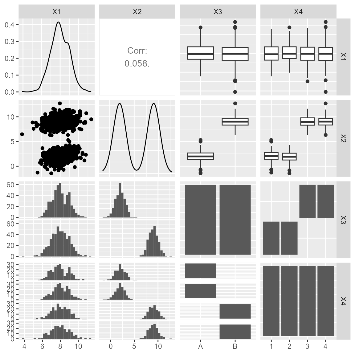
Example 1
We can fit the DPMM with missing data in “X1”/“X3” present in the original dataset. Let’s introduce some misisngness in both clusters.
dataset_missing <- dataset_5
dataset_missing[1,"X1"] <- NA
dataset_missing[2,"X3"] <- factor(NA, levels = levels(dataset_5[,"X3"]))
Then we fit the DPMM whilst standardising values.
posteriors <- runModel(dataset_missing,
                       mcmc_iterations = 2500,
                       L = 6,
                       mcmc_chains = 2,
                       standardise = FALSE)
#> ===== Monitors =====
#> thin = 1: alpha, logDens, muL, phiL, tauL, v, x_cont_miss, x_disc_miss, z
#> ===== Samplers =====
#> sumLogPostDens sampler (1)
#>   - logDens
#> RW_wishart sampler (1)
#>   - R1[1:2, 1:2]
#> RW sampler (2)
#>   - alpha
#>   - kappa1
#> posterior_predictive sampler (1)
#>   - x_disc_miss[]  (1 element)
#> conjugate sampler (29)
#>   - v[]  (5 elements)
#>   - phiL[]  (12 multivariate elements)
#>   - muL[]  (6 multivariate elements)
#>   - tauL[]  (6 multivariate elements)
#> conditional_RW sampler (1)
#>   - x_cont_miss[1, 1:2]
#> categorical sampler (1000)
#>   - z[]  (998 elements)
#>   - zmiss[]  (2 elements)
#> |-------------|-------------|-------------|-------------|
#> |-------------------------------------------------------|
#> |-------------|-------------|-------------|-------------|
#> |-------------------------------------------------------|
And we can check how well are those missing values being imputed during the model fitting. Here, we are only checking chain 1, but it can be repeated for all other chains.
imputed_values <- as_tibble(posteriors$samples$chain1)%>%
  select(`x_cont_miss[1, 1]`)%>%
  dplyr::slice(1000:2500)%>%
  unlist()
ggplot() +
  geom_density(aes(x = imputed_values)) +
  geom_vline(aes(xintercept = dataset_5[1,"X1"]))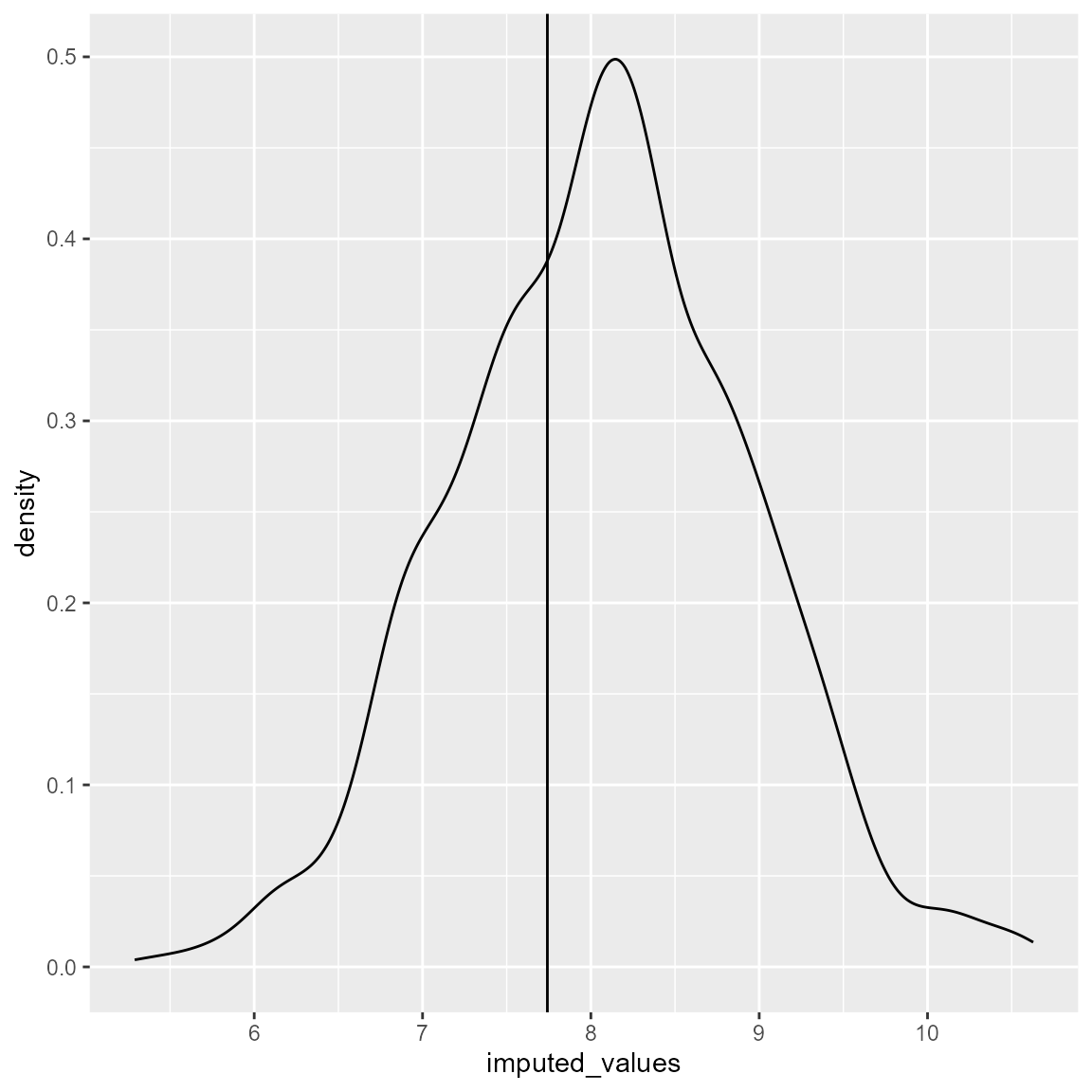
Example 2
We can fit the DPMM with missing data in ‘X1’/‘X2’/‘X3’ present in the original dataset. Let’s introduce some misisngness in both clusters.
dataset_missing <- dataset_5
dataset_missing[1,c("X1", "X2")] <- NA
dataset_missing[1,"X3"] <- factor(NA, levels = levels(dataset_5[,"X3"]))
Then we fit the DPMM whilst standardising values.
posteriors <- runModel(dataset_missing,
                       mcmc_iterations = 2500,
                       L = 6,
                       standardise = FALSE)
#> ===== Monitors =====
#> thin = 1: alpha, logDens, muL, phiL, tauL, v, x_cont_miss, x_disc_miss, z
#> ===== Samplers =====
#> sumLogPostDens sampler (1)
#>   - logDens
#> RW_wishart sampler (1)
#>   - R1[1:2, 1:2]
#> RW sampler (2)
#>   - alpha
#>   - kappa1
#> posterior_predictive sampler (2)
#>   - x_disc_miss[]  (1 element)
#>   - x_cont_miss[1, 1:2]
#> conjugate sampler (29)
#>   - v[]  (5 elements)
#>   - phiL[]  (12 multivariate elements)
#>   - muL[]  (6 multivariate elements)
#>   - tauL[]  (6 multivariate elements)
#> categorical sampler (1000)
#>   - z[]  (999 elements)
#>   - zmiss[]  (1 element)
#> |-------------|-------------|-------------|-------------|
#> |-------------------------------------------------------|
#> |-------------|-------------|-------------|-------------|
#> |-------------------------------------------------------|
And we can check how well are those missing values being imputed during the model fitting. Here, we are only checking chain 1, but it can be repeated for all other chains.
imputed_values_1 <- as_tibble(posteriors$samples$chain1)%>%
  select(`x_cont_miss[1, 1]`)%>%
  dplyr::slice(1000:2500)%>%
  unlist()
imputed_values_2 <- as_tibble(posteriors$samples$chain1)%>%
  select(`x_cont_miss[1, 2]`)%>%
  dplyr::slice(1000:2500)%>%
  unlist()
ggplot() +
  geom_point(aes(x = imputed_values_1, y = imputed_values_2), alpha = 0.6) +
  geom_point(aes(x = dataset_5[1,"X1"], y = dataset_5[1,"X2"]))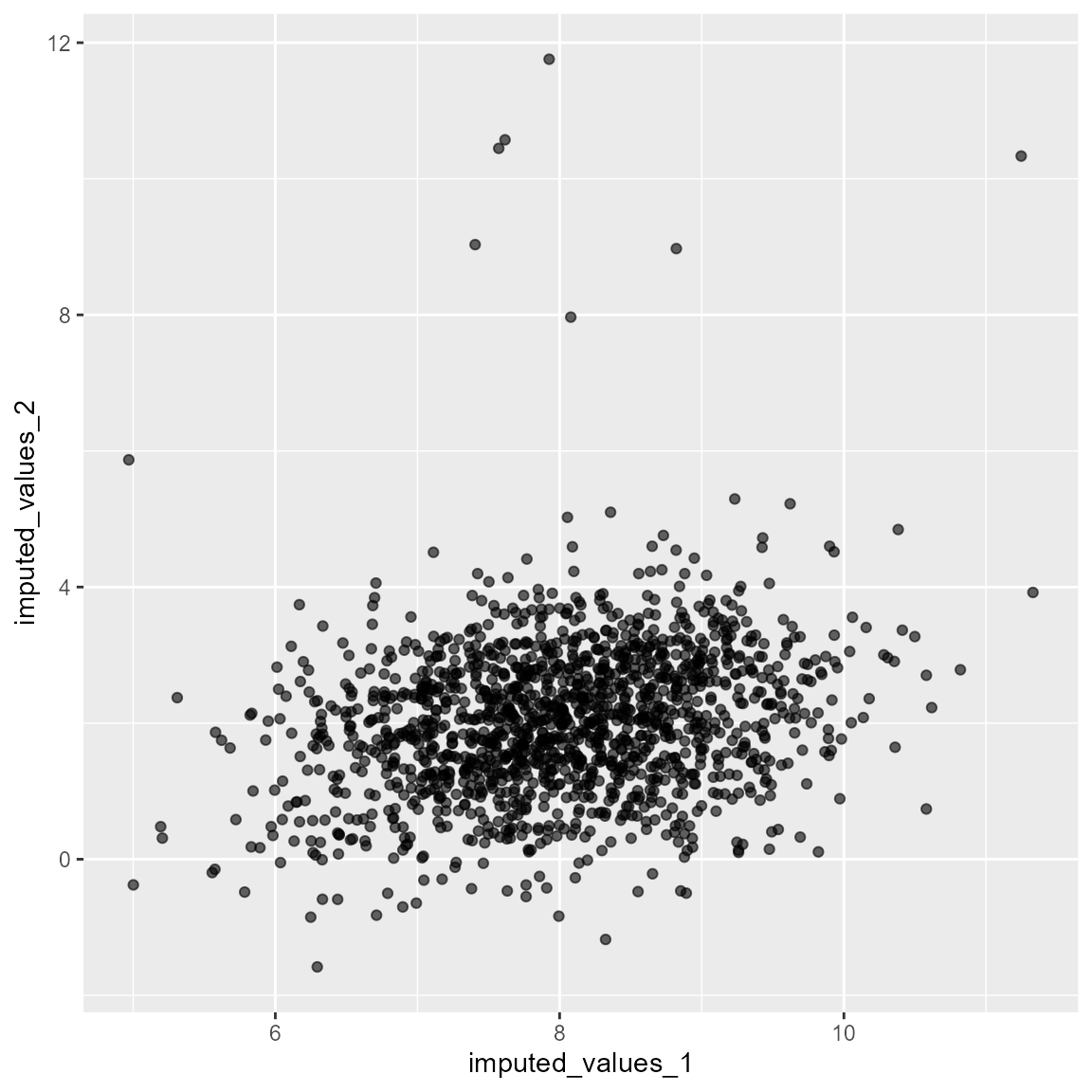
# Table predicted values vs observed values
# Note: Variable X3 is well explained by X4
imputed_values <- as_tibble(posteriors$samples$chain1)%>%
        select(`x_disc_miss[1, 1]`)%>%
        dplyr::slice(1000:2500)%>%
        unlist()
cbind(imputed_values, rep(dataset_5[1,"X3"], rep = 1500)) %>%
  as.data.frame() %>%
   rlang::set_names(c("Predicted","True")) %>%
  table()
#>          True
#> Predicted    1
#>         1 1487
#>         2   14
Example 3
We can fit the DPMM with missing data in ‘X1’/‘X3’/‘X4’ present in the original dataset. Let’s introduce some misisngness in both clusters.
dataset_missing <- dataset_5
dataset_missing[1,"X1"] <- NA
dataset_missing[1,"X3"] <- factor(NA, levels = levels(dataset_5[,"X3"]))
dataset_missing[1,"X4"] <- factor(NA, levels = levels(dataset_5[,"X4"]))
Then we fit the DPMM whilst standardising values.
posteriors <- runModel(dataset_missing,
                       mcmc_iterations = 2500,
                       L = 6,
                       standardise = FALSE)
#> ===== Monitors =====
#> thin = 1: alpha, logDens, muL, phiL, tauL, v, x_cont_miss, x_disc_miss, z
#> ===== Samplers =====
#> sumLogPostDens sampler (1)
#>   - logDens
#> RW_wishart sampler (1)
#>   - R1[1:2, 1:2]
#> RW sampler (2)
#>   - alpha
#>   - kappa1
#> posterior_predictive sampler (2)
#>   - x_disc_miss[]  (2 elements)
#> conjugate sampler (29)
#>   - v[]  (5 elements)
#>   - phiL[]  (12 multivariate elements)
#>   - muL[]  (6 multivariate elements)
#>   - tauL[]  (6 multivariate elements)
#> conditional_RW sampler (1)
#>   - x_cont_miss[1, 1:2]
#> categorical sampler (1000)
#>   - z[]  (999 elements)
#>   - zmiss[]  (1 element)
#> |-------------|-------------|-------------|-------------|
#> |-------------------------------------------------------|
#> |-------------|-------------|-------------|-------------|
#> |-------------------------------------------------------|
And we can check how well are those missing values being imputed during the model fitting. Here, we are only checking chain 1, but it can be repeated for all other chains. First we check ‘X3’, which is well explained by ‘X2’.
imputed_values <- as_tibble(posteriors$samples$chain1)%>%
  select(`x_disc_miss[1, 1]`)%>%
  dplyr::slice(1000:2500)%>%
  unlist()
cbind(imputed_values, rep(dataset_5[1,"X3"], rep = 1500)) %>%
  as.data.frame() %>%
   rlang::set_names(c("Predicted","True")) %>%
  table()
#>          True
#> Predicted    1
#>         1 1500
#>         2    1
Then we check ‘X4’, which is well explained by ‘X2’ but should have two categories.
imputed_values <- as_tibble(posteriors$samples$chain1)%>%
  select(`x_disc_miss[1, 2]`)%>%
  dplyr::slice(1000:2500)%>%
  unlist()
cbind(imputed_values, rep(dataset_5[1,"X4"], rep = 1500)) %>%
  as.data.frame() %>%
   rlang::set_names(c("Predicted","True")) %>%
  table()
#>          True
#> Predicted   1
#>         1 751
#>         2 744
#>         3   3
#>         4   3
Then we check ‘X1’, which is well explained by ‘X2’.
imputed_values <- as_tibble(posteriors$samples$chain1)%>%
  select(`x_cont_miss[1, 1]`)%>%
  dplyr::slice(1000:2500)%>%
  unlist()
ggplot() +
  geom_density(aes(x = imputed_values)) +
  geom_vline(aes(xintercept = dataset_5[1,"X1"]))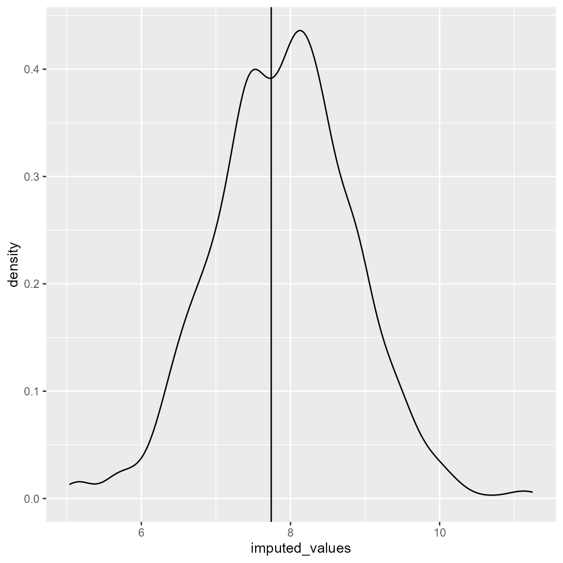
Dataset 6
Dataset 5 is comprised of two distinct clusters, where the values of both predictors do not overlap each other. The clusters are defined so that they have a specific shape.
Example 1
We can fit the DPMM to the complete dataset.
posteriors <- runModel(dataset_6,
                       mcmc_iterations = 2500,
                       L = 6,
                       standardise = FALSE)
#> ===== Monitors =====
#> thin = 1: alpha, logDens, muL, tauL, v, z
#> ===== Samplers =====
#> sumLogPostDens sampler (1)
#>   - logDens
#> RW_wishart sampler (1)
#>   - R1[1:2, 1:2]
#> RW sampler (2)
#>   - alpha
#>   - kappa1
#> conjugate sampler (17)
#>   - v[]  (5 elements)
#>   - muL[]  (6 multivariate elements)
#>   - tauL[]  (6 multivariate elements)
#> categorical sampler (1000)
#>   - z[]  (1000 elements)
#> |-------------|-------------|-------------|-------------|
#> |-------------------------------------------------------|
#> |-------------|-------------|-------------|-------------|
#> |-------------------------------------------------------|
We then check the fit of the DPMM versus the original data.
plot_ggpairs(posteriors,
             newdata = dataset_6,
             nburn = 1500)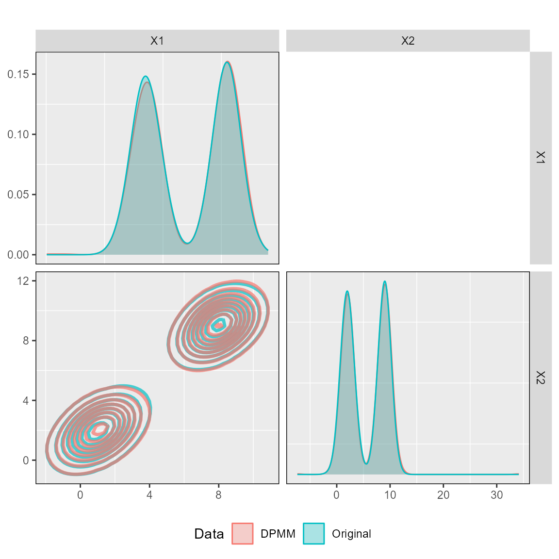
We can introduce missingness in the dataset and check whether the DPMM is predicting values correctly. In this case, we introduce missingness in ‘Y’ for 100 random patients.
rows <- 1:50
dataset_missing <- dataset_6
dataset_missing_predict <- dataset_missing[rows,]
dataset_missing_predict[,"X1"] <- as.numeric(NA)
And make predictions from the fitted DPMM.
posteriors.prediction <- predict_dpmm_fit(posteriors,
                                          dataset_missing_predict,
                                          samples = seq(1500,2500, 25))
We can then check whether the values are being predicted in the right place.
low_q <- NULL
median_q <- NULL
high_q <- NULL
for (i in 1:length(posteriors.prediction)) {
  low_q <- c(low_q, quantile(unlist(posteriors.prediction[[i]][]), probs = c(0.05)))
  median_q <- c(median_q, quantile(unlist(posteriors.prediction[[i]][]), probs = c(0.5)))
  high_q <- c(high_q, quantile(unlist(posteriors.prediction[[i]][]), probs = c(0.95)))
}

cbind(dataset_6[rows,"X1"],low_q, median_q,high_q) %>%
  as.data.frame() %>%
   rlang::set_names(c("observed", "low","median","high")) %>%
  ggplot() +
  geom_point(aes(x = observed, y = median)) +
  geom_errorbar(aes(x = observed, ymin = low, ymax = high)) +
  geom_abline(aes(intercept = 0, slope = 1))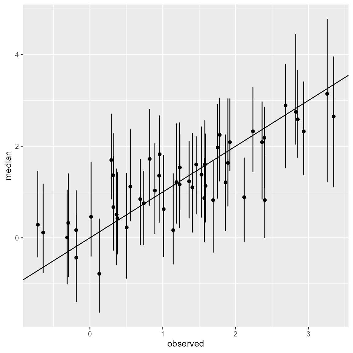
Example 2
We can fit the DPMM with missing data in ‘X1’ present in the original dataset. Let’s introduce some misisngness in both clusters.
dataset_missing <- dataset_6
dataset_missing[1,"X1"] <- NA
dataset_missing[501,"X1"] <- NA
Then we fit the DPMM whilst standardising values.
posteriors <- runModel(dataset_missing,
                       mcmc_iterations = 2500,
                       L = 6,
                       standardise = FALSE)
#> ===== Monitors =====
#> thin = 1: alpha, logDens, muL, tauL, v, x_cont_miss, z
#> ===== Samplers =====
#> sumLogPostDens sampler (1)
#>   - logDens
#> RW_wishart sampler (1)
#>   - R1[1:2, 1:2]
#> RW sampler (2)
#>   - alpha
#>   - kappa1
#> conjugate sampler (17)
#>   - v[]  (5 elements)
#>   - muL[]  (6 multivariate elements)
#>   - tauL[]  (6 multivariate elements)
#> conditional_RW sampler (2)
#>   - x_cont_miss[1, 1:2]
#>   - x_cont_miss[2, 1:2]
#> categorical sampler (1000)
#>   - z[]  (998 elements)
#>   - zmiss[]  (2 elements)
#> |-------------|-------------|-------------|-------------|
#> |-------------------------------------------------------|
#> |-------------|-------------|-------------|-------------|
#> |-------------------------------------------------------|
And we can check how well are those missing values being imputed during the model fitting. Here, we are only checking chain 1, but it can be repeated for all other chains.
imputed_values <- as_tibble(posteriors$samples$chain1)%>%
  select(`x_cont_miss[1, 1]`)%>%
  dplyr::slice(1000:2500)%>%
  unlist()
ggplot() +
  geom_density(aes(x = imputed_values)) +
  geom_vline(aes(xintercept = dataset_6[1,"X1"]))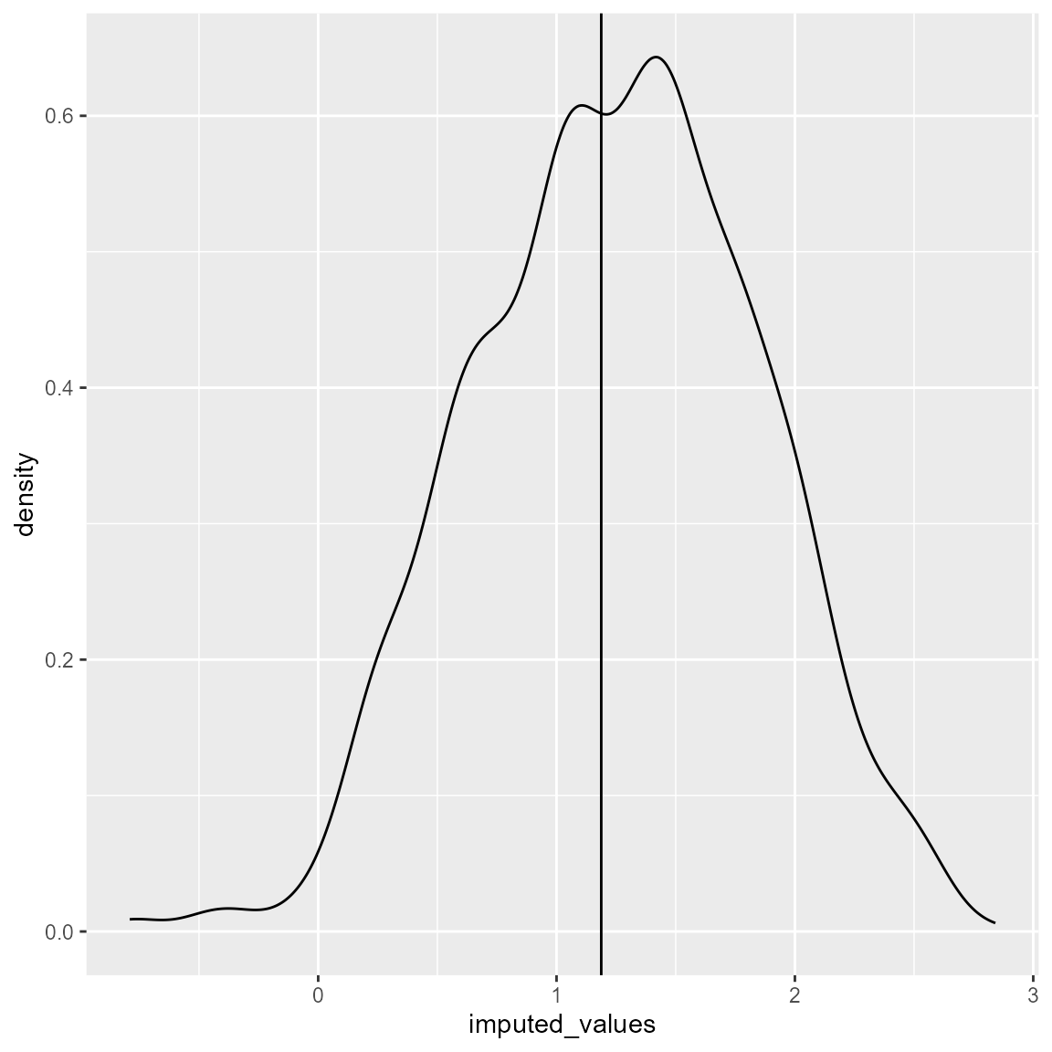
imputed_values <- as_tibble(posteriors$samples$chain1)%>%
  select(`x_cont_miss[2, 1]`)%>%
  dplyr::slice(1000:2500)%>%
  unlist()
ggplot() +
  geom_density(aes(x = imputed_values)) +
  geom_vline(aes(xintercept = dataset_6[501,"X1"]))